Probability
Why do we care about probability?
Before we introduce statistical distributions like the normal distribution, we need a way to talk about uncertainty.
In agriculture and biological systems:
Outcomes vary
Measurements are never identical
We rarely know exact future values
Probability gives us a language to describe how likely different outcomes are. I like to think of probability as a way of counting the number of different ways a given event can happen within a system.
An example would be, in a given corn field in a given year:
- How likely are we to measure an average yield throughout the field above 180 bu/ac?
This question can be stated again as:
- How many scenarios out of all possible scenarios for this field can the average be above 180 bu/ac?
To answer this question, we need to understand how yield values vary and how frequently different values occur. We are going to talk about this soon! First, let me do a brief detour to explain some important concepts.
A brief non-agronomic example
Defining probability
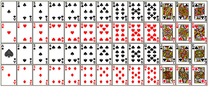
To think of probability as a way of counting the occurrence of a given scenario within all possible scenarios, I believe it is useful to think of a case in which there is a limit to the number of scenarios: a deck of cards!
By this definition, we can think of probability of event \(x\) happening as:
\[ Pr(x) = \frac{n}{N}\]
Using this framework, let’s think of the probability of drawing an ace from an ordinary deck of 52 playing cards:
Since there are 4 aces (\(n=4\)), among the 52 cards (\(N=52\)), the probability of drawing an ace is \(4/52\) or \(1/13\).
Some simple rules of probability
Probability does not tell us what will happen in a single case; it describes patterns across many possible cases.
Limits
If we’re thinking of counting ways that an event could happen among all possible events, the lower limit for how probable an event is would for this event to simply never happen among all scenarios. This would result in \(n=0\). As a result, regardless of the value of \(N\), we have:
\[Pr(x) = \frac{0}{N} = 0\]
Similarly, for the upper bound, the most this event could happen is in every possible scenario. Thus, \(n=N\). This results in:
\[Pr(x) = \frac{N}{N} = 1\]
Complementary events
The same way we are counting the number of times an event could happen among all scenarios (like our ace among all 52 cards), we can think of the number of times all other events could happen, except for this one. For example, what is the probability of not drawing an ace?
There are 48 cards that do not represent an ace, therefore, the probability is \(48/52\) or \(12/13\).
Since when you draw a card you are going to draw either an ace or any other card, the probability of drawing an ace (\(1/13\)) or any other card (\(12/13\)) must add up to 1. Therefore:
\[Pr(not~x) = 1 - Pr(x)\]
This idea will be especially useful later when we talk about probabilities above or below a threshold, such as yield exceeding a certain value.
Probability distributions
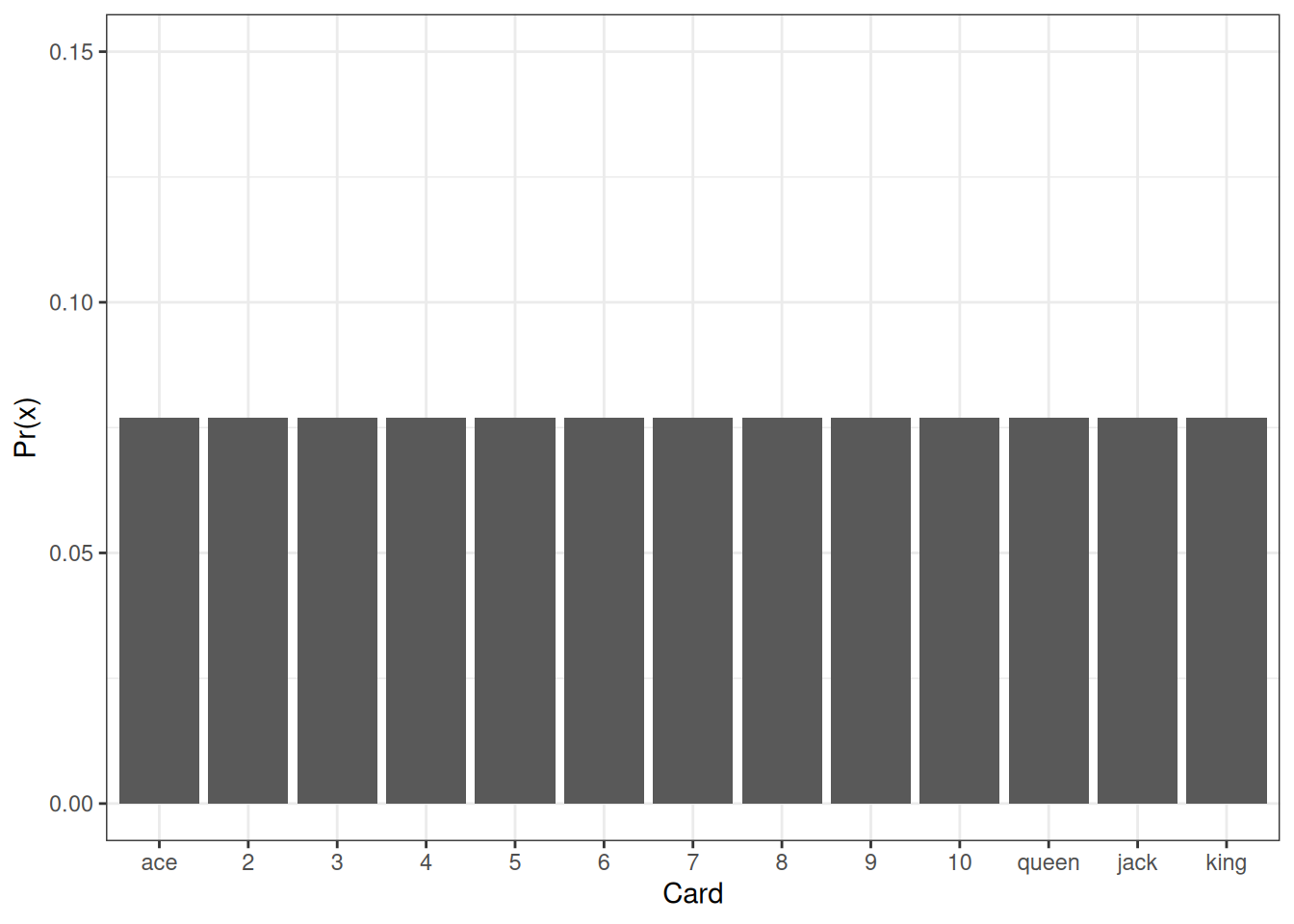
We can visualize the distribution of the probability values according to the cards in the graph below. Assuming this is an ordinary deck of cards, all cards have the same probability of being draw. That’s why the graph showing the probability is so boring!
If we sum the area of all of these bars, they should add up to 1! That’s a fundamental concept of probability distributions that we will use on more complex systems but that can be easily visualized here. If you are familiar with calculus, would this be similar to computing the area under the curve?
The mathematical formula representing this system is:
\[Pr(x) = 1/13,~for~x=ace,2,3,\ldots,king\]
Back to agronomy!
Ok, so natural systems, such as agricultural fields, are not as simple as a deck of cards, right? I believe that’s a good thing, otherwise we’d all be out of a job! In agronomic systems, we will often use more complex probability distributions to model the randomness of data, but the concepts we have just learned are going to remain the same!
The normal distribution
One commonly used probability distribution in agriculture is the normal distribution. It describes situations where values tend to cluster around an average, with fewer observations far from the mean. Take a look at the graph below.
In the card example, outcomes were discrete and countable. However, yield is a continuous variable, and it can take on many possible values within a range. For continuous variables, probabilities are described using probability density rather than simple counts.
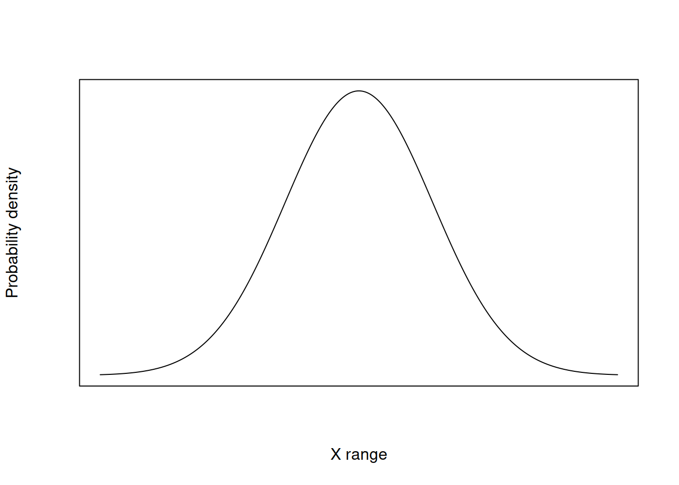
The height of the curve at any point is not a probability by itself. Probabilities come from the area under the curve over a range of values. In the case of the deck of cards, adding up the area of the bars was equal to one. Here, that’s also true. Except that, for continuous variables, to compute the area under the curve, we need to integrate over \(X\). We will not cover this more advanced calculus tasks in this class, but I wanted you to have an intuition for it.
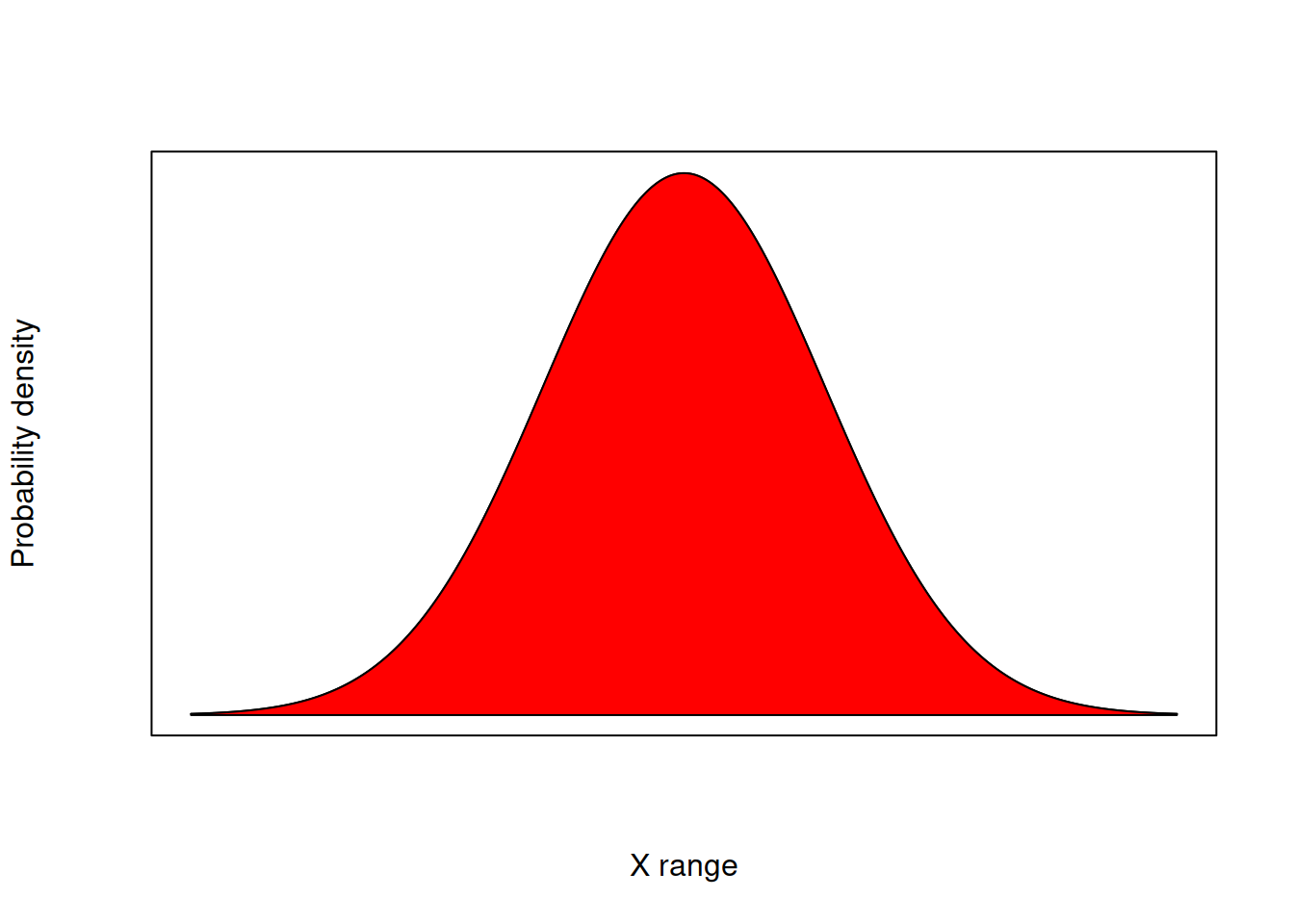
Therefore, the red shaded area in the figure below has an area equal to 1. This means that the probability of \(x\) assuming any value possible is 1. In the case of the deck of cards, it would be the equivalent of asking “What is the probability of the card I drew being a card?”. Sounds silly, I know!
Normal distribution
I do not want to scare you with this equation! But I thought you might like to see the equation that describes the shape above! Also, note that the entire equation can be described with \(\mu\) and \(\sigma\). These represent the distribution’s mean and standard deviation. These two distribution parameters represent the center and the spread of the normal distribution. We’ll talk more about it soon!
\[f(x|\mu,\sigma) = \frac{1}{\sigma \sqrt{2\pi}} \exp\left( -\frac{(x - \mu)^2}{2\sigma^2} \right)\]
Case study
Soybean yield data
Ok, so I spent some time now talking about the probabilities and distributions until now. Let’s take a look at how this applies to our case. We’ll load up some simulated yield data from a soybean field. Let’s take a look at the yield map:
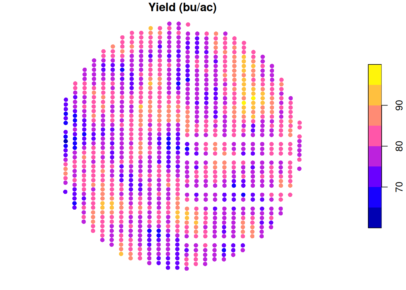
This data contains 1038 observations and we can see that it varies between 64.52 and 96.54 bu/ac, averaging about 79.82 bu/ac. Not bad!
length(yield)[1] 1038summary(yield) Min. 1st Qu. Median Mean 3rd Qu. Max.
64.52 76.45 79.60 79.82 82.98 96.54 Let’s take a look at how our data is distributed across yield values. Yield values can present a bell shape distribution but can also be skewed towards one way or another. For this conceptual explanation, we will assume that the normal distribution model is a good representation of the randomness of yield data.
hist(yield, xlab = 'Yield (bu/ac)')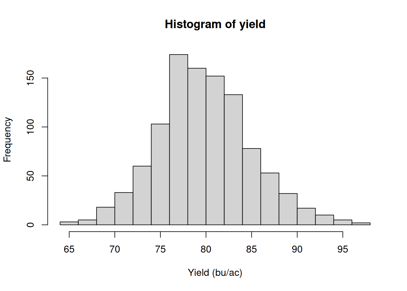
Connecting the histogram to the normal distribution
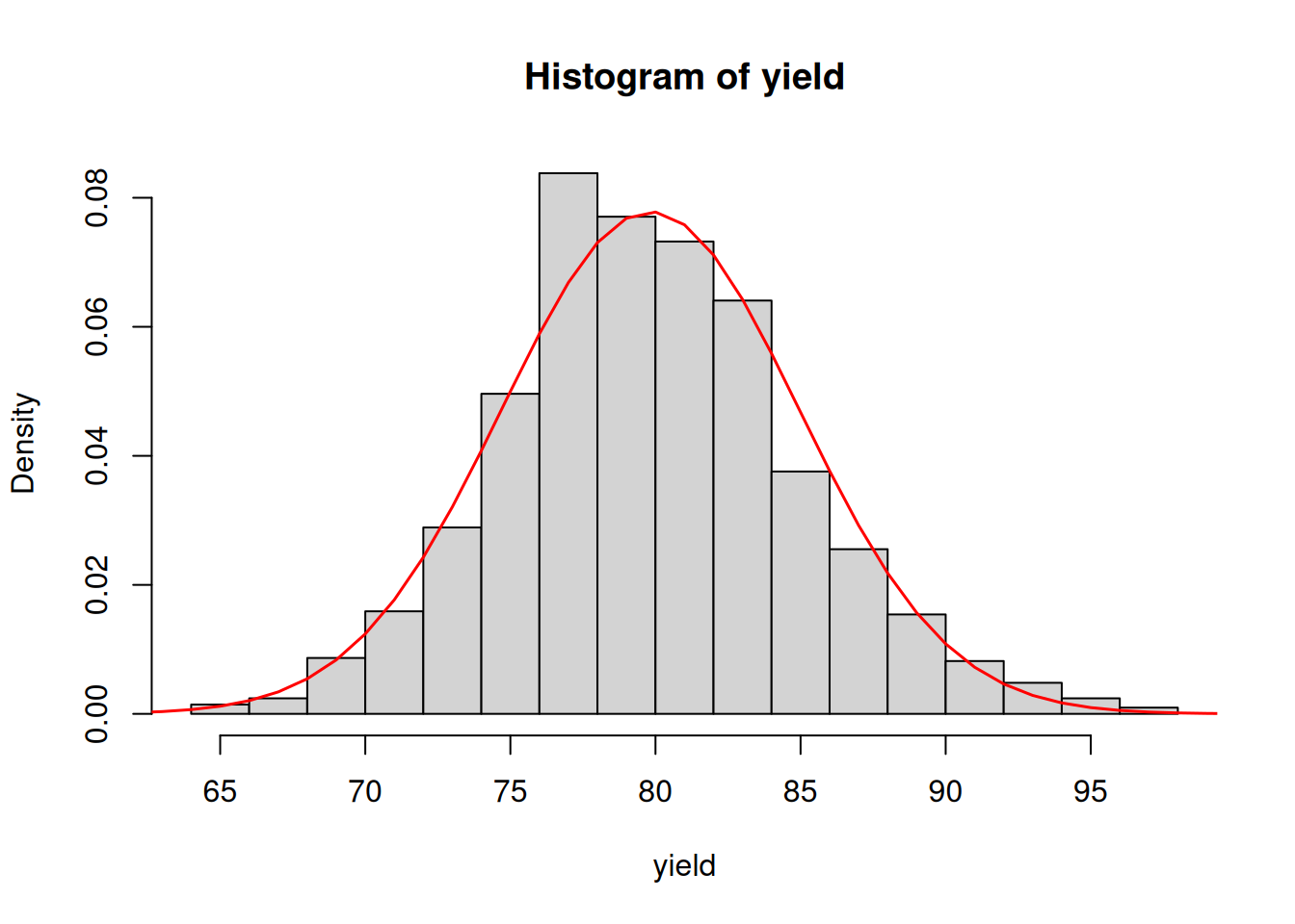
Ok, so let’s compute the mean (\(\mu\)) and the standard deviation (\(\sigma\)) of the yield data so that we can check that the normal distribution would be a good model to represent our yield data.
mean(yield)[1] 79.82476sd(yield)[1] 5.12554Using the mean and the standard deviation (and that ugly equation from before!!!), we can place the normal distribution model on top of our histogram. We can see that it’s a good fit. It’s not perfect because it’s a model but it can tell us many interesting things about the data, as we’ll see in the next steps.
A side note, the normal distribution model tells us a lot about what to expect from the data in terms of which values will be more likely to be observed and which will be less likely. However, it does not tell us something like: Oh, the yield in this field will always be 79 bu/ac.
Computing probabilities
Something that the normal distribution model allows us to do, is to check compute the probability of a given value falling within a range, right? Just like adding the area of the bars in the deck of cards example, if we integrate over \(X\) between two values, we can check the probability of observing a value of \(X\) within those ranges. Let’s check the probability of getting a value between 70 and 80 bushels!
The red shaded area is represents a probability of about 48.6% of the yield value falling between these bounds.
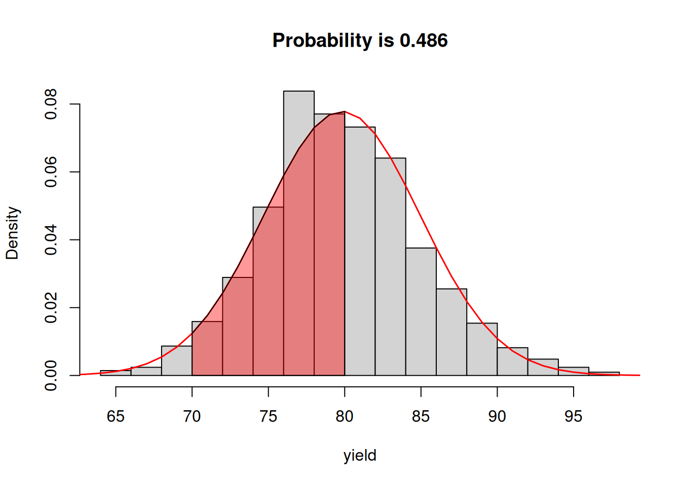
We can check that the normal distribution model is a good representation of our data by looking at the number of data points between these bounds as well. The code below shows that counting the data has a proportion of 51% of the data between those bounds. Not perfect but pretty close!
N <- length(yield)
yield_values_within_bounds <- yield[yield >= 70 & yield <= 80]
n <- length(yield_values_within_bounds)
n / N
[1] 0.5105973The standard normal distribution
The standard normal distribution model is probably one of the most used in statistics. Now that we have learned the properties of the normal distribution, how about we generalize these properties to a standardized version of the distribution?
The standard normal distribution corresponds to a normal distribution in which \(\mu = 0\) and \(\sigma = 1\). The way to do it is to standardize the data is to subtract the mean and divide by the standard deviation, like this:
\[Z = \frac{x - \mu}{\sigma}\]
Once we standardize the data, we usually call it \(Z\). This is also why the standard normal can be called the Z distribution. This is useful because it centers the data at 0 and allows us to talk about the spread of the data in terms of standard deviations. Let’s take a look at some of these rules of thumb.
The 68%, 95%, and 99% rule
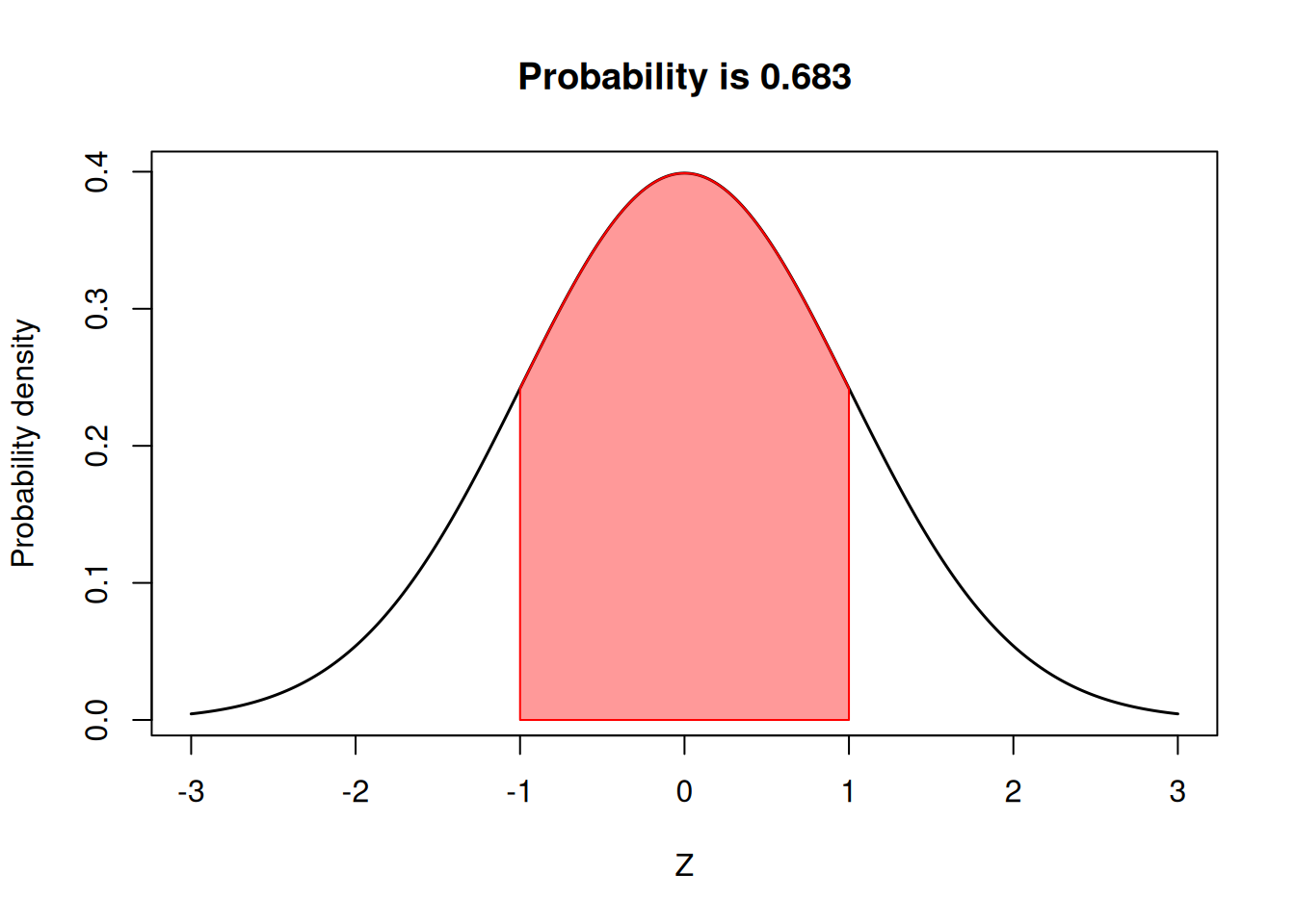
68% probability or \(1\sigma\)
Now that we have standardized the normal distribution, we can think of it in terms of how many standard deviations from the mean a given value is. What is the probability of a value being within \(1\sigma\) of the mean? Let’s compute is!
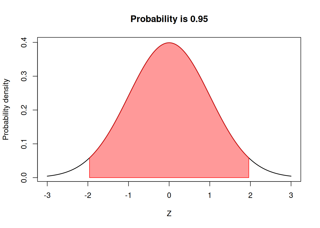
95% Probability or \(1.96\sigma\)
One of the most common hard-set thresholds in statistics is to compare means or treatments, or compute confidence intervals at a 5% tolerance. Have you heard of it? 95% of the area of the curve is within \(1.96\sigma\).
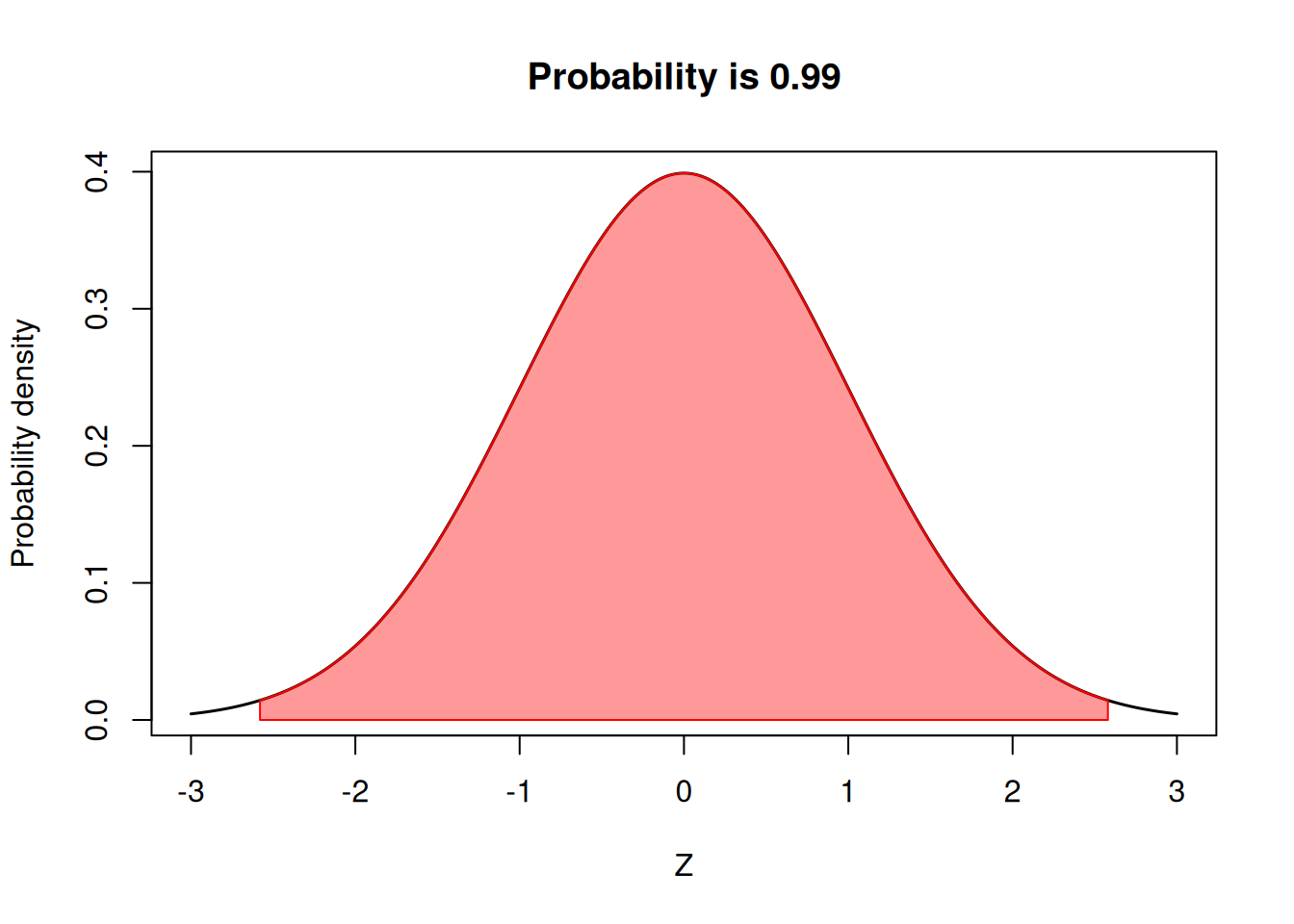
99% Probability or \(2.58\sigma\)
At times, we might want to be more cautious about finding differences. For example, when we are trying to identify whether a herbicide might cause injury to the crop. This is a situation in which a wrong test might cost a lot of money to the producer or the company. In that case, we might want to make our standards a little more strict to identify differences between treatments. Therefore, we might be interested in which values would correspond to 99% of the probability. That value corresponds to \(2.58\sigma\).
Looking into the future
We have just learned the origin of important numbers in population statistics. As we get further into this course, we will learn about other distributions, such as binomial and F, and the unique tests in which they are used. Even in those cases, some of these concepts will stay the same: identifying whether the observed values are likely to occur (happening within those 95% or 99% bounds) or if they are unusual values (happening within the remaning 5% or 1% of the distribution).